


It can be really hard to keep track of the work you do without creating reports in some way. Like you would in a wet lab environment, working on analyses on your computer requires some way to track what you have done, and when you did it. While the easiest ways to do this are by using comprehensive version control software, often, your smaller analyses don’t really need such verbose options. Being able to keep a record of your code, when you ran it and how you set up your environment before running it is key in being able to reproduce your results.
Markdown is an easy to use feature in R that will save your code and output, both textually and visually, to a PDF or HTML file for easy access. You can include the date, author and version information, as well as text explanations of your code in whatever format makes most sense to you.
If you are looking for a way to create a coding “lab book” then you can utilise Markdown in R. Here, we explain the basics of R Markdown and knitr.
Create a New Document
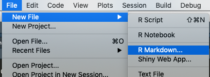
Create your R Markdown document in R Studio. In the File menu, find the option for New File, then choose R Markdown.
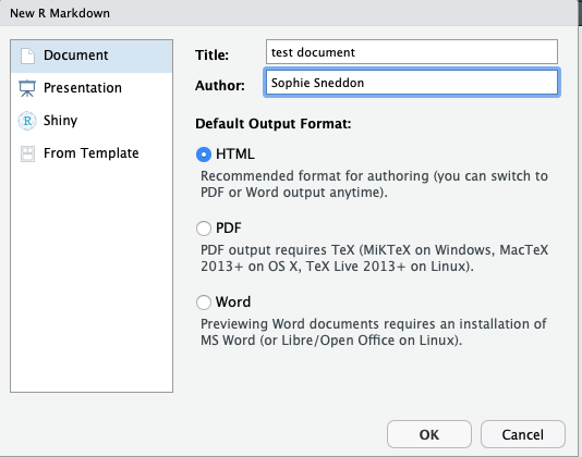
A window will open allowing you to name the document and choose the settings associated with it. Here, you can also choose the output format.
Enter Document Information
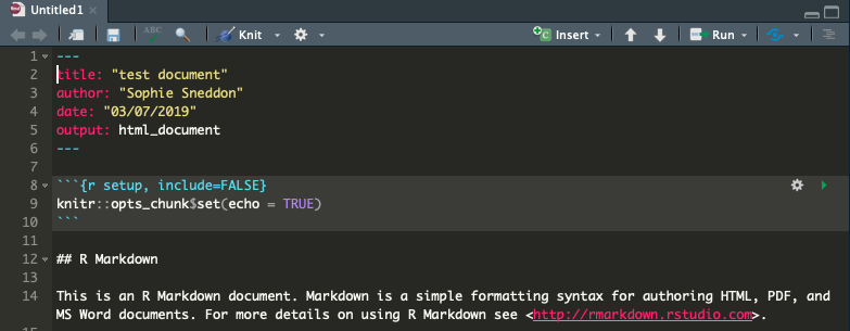
Now that you a brand new R Markdown document, it is important to make sure everything is correct at the top. If you are working on an older file, make sure you change the date so that the information is correct when you create your new HTML or PDF file.
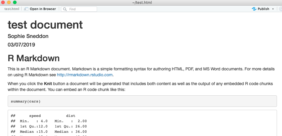
R Studio has provided you with a sample template that contains a brief tutorial using the mtcars data to show you how to use the simple formatting options. You can run this template straight away by clicking on the knit button at the top of the Source pane. You will be asked where you would like to save the file, so choose a location and let the script run. I’ve chosen HTML, so a window will pop up with my new page containing the output.
You can see that the template explains simple formatting, but we will go over it here as well.
Simple Formatting
R Markdown utilises a number of easy formatting methods that enable you to highlight certain aspects of the text that is displayed with your code and output. These formatting options are similar to many popular text based communications platforms, such as Slack, Discord and Reddit. Here are a few of the most useful options.
Headers
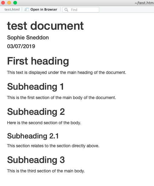
Separating your data using headings is a good way to provide structure and organisation to the final product. You can add headers using the # symbol. The more # you place before your header text, the smaller the heading becomes. For example:
# First heading

This text is displayed under the main heading of the document.

## Subheading 1

This is the first section of the main body of the document.

## Subheading 2

Here is the second section of the body.

### Subheading 2.1

This section relates to the section directly above.

## Subheading 3

This is the third section of the main body.
A good rule of thumb for formatting any type of document is to maintain the header hierarchy. Below, you can see that the output of the above code results in headers that become smaller depending on the number of # used before the heading.
Text Formatting
Add style and formatting to your text with these quick options:
Bold: *bold text*
Italics: **italic text**
Strikethrough: –striked text–
Superscript: ^superscript text^
Links: [link](google.com)
Block text: >text here
Code Chunks
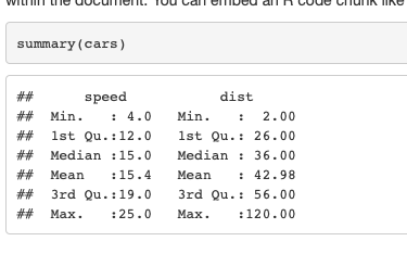
The code is the guts of your document. Where you would normally add R code within your script, you need to insert it into a code chunk in Markdown in order for it to be properly parsed. Code chunks are created by placing three back ticks (“`) at the beginning and end of the chunk. The code chunk must be uniquely named, which you can do by including the name in curly brackets after the first set of back ticks. The first code chunk in the example Markdown file created by R when you open a new document shows this in action:
```{r cars}
summary(cars)
```
You can put any R code within the code chunk, and the output will be displayed in-line. Here is the output of the above chunk:
Output Options
The output of your code chunks can be controlled by using particular options within your opening tags. The options are explained below.
echo=FALSE: This tag restricts your code from being output into the final markdown document. However, this will not prevent the results from being shown.
message=FALSE: This tag ensures that any system messages are excluded from the final output.
warning=FALSE: Warnings can sometimes have no affect on your final result. This tag will restrict the warnings from being displayed in your final output.
fig.cap=”<caption>”: This tag will add a caption to the figure generated from the block of code.
include=FALSE: This tag restricts all output including code and results included and generated from the corresponding block.
Options can be added in the following way:
```{r code_example, echo=FALSE}
# the code and output of this code chunk is suppressed
```
Conclusion
This guide is a simple example of how to get started using R Markdown. Creating markdown documents is an intuitive way to document and record what you have done in R and is very easy to use. There are more options and formatting techniques you can use to insert images, equations, tables, lists and more into your document that will be featured in future tutorials. For now, you can view the official R cheatsheet so that you can quickly find these options when you need them. Happy coding!
Disclaimer: This tutorial is designed to offer quick solutions to common problems. They do not necessarily represent the most efficient way to perform the tasks outlined.


